STM 308

Linear Equations and Systems

A Linear equation has some set of variables.

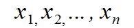
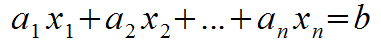
These variables are an equation of the form:

Why Linear?

Because we don't deal with curves. No spheres. No parabolas.

The number of variables the system has determines the number of dimensions the resulting solution will have.

• R² means 2 variables (n = 2) so it's a line but results in a point.
• R³ means 3 variables, so it's a plane but results in a line.
• R⁴ means 4 variables, so it's a hyper-plane (?), but results in a cube.

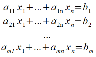
Linear System

See Linear System Definition

Example:

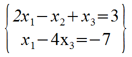
In this system, there are 2 equations and 3 unknowns. The size of this system is 2 by 3 (2x3). 4x5 is 4 equations, 5 unknowns.

Refer to the columns as x₁ column, and solution column.

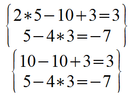
An example solution is the triple (5, 10, 3).

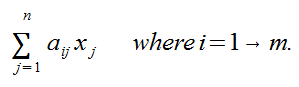
The long form of Rⁿ systems are:

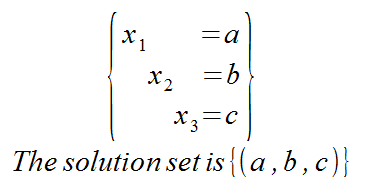
The solution is expressed as:

Row Operations

Row Interchange

R_i (Row-number (equation number) ← R_j.

Swap row-i and row-j

Undo: R_i ← R_j

Row Scaling

R_i ← cR_i where c ≠ 0

When c=0, this removes an equation thus creates a new system.

Undo: R_i ← 1/c R_i

Row Replacement

R_i ← R_i + C R_j

C can be 0, but that's complicated, so avoid it.

Undo: R_i ← R_i - C R_j

Here is the simplest, easiest, solved Linear System that's a size of 3x3:

Any other 3x3 Linear System can be transformed into this System using the row operations.

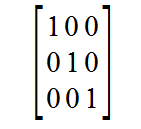
A much cleaner verison excludes the variables. This is called a coefficient Matrix and it looks much more similar to happy matricies of youth and 3D programming.

Row operations are reversible.

Inconsistent solutions

If the augmented form of a Linear System has a row of the for [0 ... 0 | b] where b ≠ 0, then the Linear System is consistent.

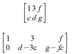
The only time this matrix is inconsistent is if d-3c == 0 and g-fc ≠ 0, because then a zero-row has a non-zero value, which is mathematically impossible.

Theory

Basic properties of real numbers.

• If a, b, c are real numbers, where c ≠ 0, then a=b ↔ ac = bc
• This goes both ways. This is how we can justify Row Scaling.
• If a, b, c, d are real numbers and a=b and c=d then a+c = b+d
• This does not go both ways. It is an if-statement. So if the result is true, it does not necicarilly mean the condition is true.

The reversibility of the row operations along with the basic properties above, ensures that the solution sets of row-equivalent linear systems are the same.

Matricies

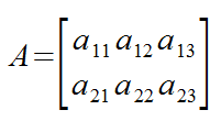
• Matricies are denoted by capital letters with the entries enclosed with square brackets.
• If A is an mxn matrix, then the entry in the (i, j)-positon is denoted by a_ij
• Matrix
• Zero Row
• Non-Zero Row
• Echelon Form
• Reduced Echelon Form

Theorem

If A is an mxn matrix, then there exists a unique matrix U in reduced echelon form such that A ~ U.

If A ~ U and U is in echelon form, then we call U an echelon form of A; if U is in reduced ecehlon form, then we call U the reduced ecehlon form of A. We specify an versus the because reduced ecehlon form is unique, but regular echelon is not unique.

Types of Solutions

Inconsistent

A zero-row has a non-zero value in the solution column.

Unique

Every column in the coefficient matrix is a pivot column.

Infinite

Presence of free variables, that is, one of the columns of the coefficient matrix is not a pivot column.

Example:

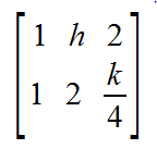
• Inconsistent if h = 2 and k ≠ 8
• Unique if h ≠ 2. k can be anything, so we don't specify it at all.
• Infinite if h = 2 and k = 8.

Vectors

• Vector Space
• Parallelogram Law
• Zero Vector

Literally just a matrix with a single column. The number of row corresponds to the number of dimensions the system is in.

Addition

Scalar Multiplication

Literally just multiply each entry by the same real number.

Translation

Algebraic Properties of Rⁿ

• Commutative. Reverse-order doesn't matter. A + B = B + A
• Associative. Doesn't matter which order you add. (A + B) + C = A + (B + C)
• A + 0 = A = 0 + A
• A + (-A) = (-A) + A = 0
• -A := -1 * A
• c(A + B) = cA + cB
• (c+d)A = cA + dA
• c(dA) = (cd)A
• 1A = A

We prove this because these properties apply to real numbers, and vector-addition is simply adding real numbers (the vector's entries), so there we go!

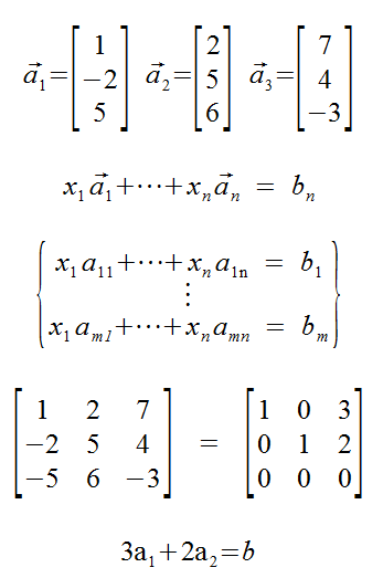
Linear Combinations

Given vectors v₁, ..., v_p in Rⁿ and scalars c₁, ..., C_p in R, the vector y is defined by:

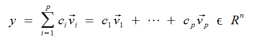
This is called the Linear Combination of v₁, ..., v_p w.r.t. the scalers c₁, ..., c_p.

We can prove that a sum of vectors multiplied by scalars can be transformed into, and thus equals, a Linear System.

Span

• Span

Properties

• Span ({v₁, ..., v_p}) contains v₁, ..., v_p.
• vector 0_m in span ({v₁, ..., v_p}). All scalars are 0 results in a zero vector.
• Determing whether vector a: [a₁ ... a_n | b] is feasible, is equal to determining whether vector b is in span({a₁, ..., a_n})

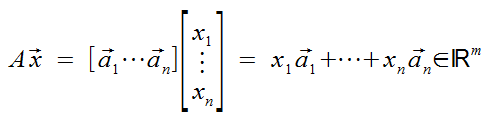
The Matrix Equation

Ax = b, where x and b are vectors.

if 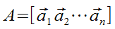is an mxn matrix & , then the product of A and vector x is defined below.

This results in transforming vectors into different dimensions unless m=n!

This is simply, nothing more, than a shorthand name for what we did with vectors above where we scaled them then added them together. This is literally a function as in programming functions. Now we just need to write Ax = b instead of that giant mess.

Even more simply put: this is vector-addition where the columns of a matrix are trated as a series of vectors, and each vector is multipled by values in another vector. The sum is our result. Easy peasy!

• Function

An mxn matrix A determines a function: T_A : Rⁿ → R^m and vector x in Rⁿ → Ax in R^m.

The "product" Ax defines a function (mapping) from Rⁿ to R^m.

T_A:Rⁿ → R^m means to send x → Ax. We are sending a vector to another dimension!

What it means to solve

Given some Matrix A, we have a destination matrix b in space R^m that we want, so we find a vector x in space Rⁿ that will result the vector b.

In 3D worlds, this means having a vertex in 4D space, multiplying it by a matrix that will result in the vertex either appearing in our 3D world, or not.

Theorem

We can find a vector b in the span of vectors a, but can we find a vector b with any value? Do some values not work? In other words, will the system be inconsistent? No. It can be inconsistent.

We need a pivot in every row of A for every vector b to be in the span of vectors a (matrix A).

The columns of A span R^m if every vector b in R^m is a linear combination of the columns of A.

Theorem

If A is an mxn matrix, then the following statements are equivalent. (they are all true, or all false).

1. Ax = b is consistent for every vector b in R^m.
2. b is in the span of vectors a
3. The columns of A span R^m (R^m = span of vectors a)
4. The Reduced Echelon Form of A has a pivot position in every row.

Theorem

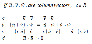
If A is an mxn matrix, then vectors u and v in Rⁿ and scalar c in R, then:

1. A(u + v) = Au + Av
2. A(cu) + c(Au)

This fails for functions like y=x², but works here because we're doing Linear algebra.

The proof is A(u+v) is equal to (u₁ v₁)a₁... Split this out to multiple u₁A₁ + v₁A₁... Now rearrange them so u's are together and v's are together, now we can pull 'u' and 'v' out to form Au Av!!

Special Tranfom Matricies

The identity matrix: taking a vector and mapping it to itself.

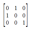
Permutation Matrix, all 1s and 0s, but in odd ways to move the values of x around. Rearrangement.

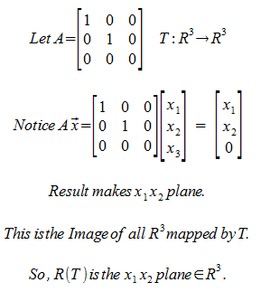
Projection Matricies. All 1s and 0s, but one row is all 0s so the x-vector will simply be projected down to a lower dimension. This is an over-simplified projection where we literally throw out a dimension of data, and the rest of the axis will be projected down.

Solution Sets of L.S.

• Homogeneous Linear System

This is an example of a homogeneous linear system and its solution. If the solution is not unique, then it is a span.

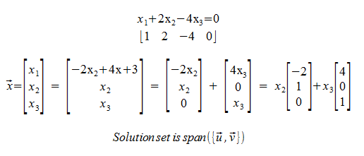
The homogeneous linear system is the base vector. That is, one that goes through the origin. Non-homogeneous linear systems are just this base linear system shifted somewhere.

Theorem

There exists vectors v₁, ..., v_p such that the solution set to Ax = 0 is span ({v₁, ..., v_p}).

Parametric Vector Equation

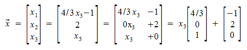
• Parametric Vector Equation

Yet another way to write down a linear system. Shows how Linear Systems can be translated. The resulting coefficient matrix is the homogeneous Linear System, and the added vector shows translation!

Theorem

Suppose Ax = b is consistent for some (maybe not all) b in R^m and let vector p in Rⁿ be a solution. Then the solution set of all Ax = b are vectors of the form w = v + p where vector v is any solution of Ax = 0.

In other words, (Ax = b) == (v + p) where p is in the span x, and v means the vector x in the homogeneous system Ax = 0.

Trivially, this vector x could always be all 0s. Non-trivially, there may be a situation where a non-zero vector results in Ax == 0. These solutions could also be used as 'v' in our simplification above.

Proof

If w = v + p, then Aw = A(v + p) = Av + Ap = 0 + b = b! Going backwards, suppose another solution to Ax = b is 's'. s = s - p + p → (s-p) + p. Notice that A(s - p) = As - Ap = b - b = 0!! Wow!

Linear (In)dependence

Remember that the Matrix Equation Ax=b is another way to write a sum of vector multiplication.

• Linearly Independent
• Linearly Dependent

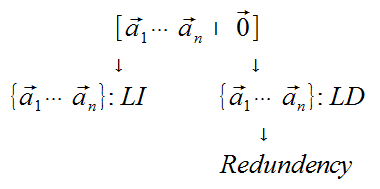
If you have a linearly dependent set, this means you have a vector in the set that's already covered in the span of those vectors. This means this vector is a linear combination of the other vectors.

What we're trying to say is that we can remove this vector without affecting the span the entire set represents.

The vectors a are linearly independent if, and only if, the homogeneous matrix A has only the trivial solution.

Example: Are the vectors below Linearly Independent? If not, find an Linear Dependence Relation.

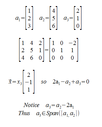
Instead of homogeneous systems with trivial or non-trivial solutions, we're looking at vectors and calling it Linearly Dependence or Linearly Independence.

Proposition

The set of a single vector v: {v}, is Linearly Independent iff the vector v does not equal 0.

The set {v₁, v₂} is L.D. iff v₁ = c v₂, where c is any constant.

Proof

(←) If v₁ = c v₂, then v₁ - c v₂ = 0, so that the set {v₁, v₂} is L.D.

(→) If {v₁, v₂} is L.D., then there exists scalars c₁ and c₂ (not both zero) such that c₁ v₁ + c₂ v₂ = 0. Assume c₁ is not 0. Then v₁ = c₂/c₁ v₂.

Theorem

The set S = {v₁, ..., v_p}, where p >= 2, is L.D. if and only if at least one of the vectors in S is a linear combination of the others.

Proof

(←) Suppose that v_j = c₁ v₁ + ... + c_j-1 v_j-1 + c_j+1 v_j+1 + ... + c_p v_p. Then 0 = c₁ v₁ + ... + c_j-1 v_j-1 - v_j + c_j+1 v_j+1 + ... + c_p v_p so that S id L.D.

(→) Suppose that S is L.D. Then there exists scalars c₁, ..., c_p (not all 0) such that c₁ v₁ + ... + c_p v_p = 0. Suppose c_j is the first non-zero scalar. Then v_j = c₁ / -1c_j v₁ + ... + what we did above. We subtract everything execpt v_j and then divide by c_j.

What we're doing here

A L.D. tells us that we have a redundency in our span of vectors, so we can remove at least one of them. And it doesn't matter which vector we remove from the span because any Linear Combination of the other vectors will still result in the same span.

Theorem

If Set S = vectors v through p in Rⁿ and p >n, then S is L.D.

Proof

The L.S. [v through v_p] is underdetermined (more columns than rows), and therefore cannot have a pivot position in every column and cannot have a unique solution.

Theorem

If S (as above) but now a Zero-Vector is in S, then S is L.D.

Proof

Assume v₁ = 0, then 1v₁ + 0v₂ + ... + 0v_p = 0.

In summary

This generalizes what we're saying, where the set of vectors either has a trivial solution for 0, or inifinite solutions for 0.

Linear Transformations

Consider a function T that maps Rⁿ into R^m. This takes some vector x in R^m and results in Ax in R^m.

When we solve a linear system Ax = b, we're just solving for this vector x to find the original vector x that results in the vector b.

• Transformations (functions)
• Image

Because T(x) = Ax, this means the same properties that apply to te Matrix Equation apply to this function T.

• T(x + y) = T(x) + T(y)
• T(cx) = c T(x)

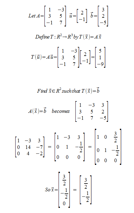
Example:

Proposition

(assuming we no nothing about T...) What is a linear transformation? What does it mean to be linear?

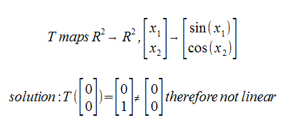
If T maps Rⁿ to R^m, then T is linear if (not only if) T(0_n) = 0_m.

If T maps Rⁿ to R^m is a function, then T is linear iff T(cx + dy) = cT(x) + dT(y)

Proof

Because T(cu) = c T(u) for every c in R, notice that T(0_n) = T(0 u) = 0 T(u) = 0_m

→ because of what we just proved above (we can take out constants/scalars).

← Because T(1x +1y) = 1T(x) + 1T(y) = T(x) + T(y). And T(cx) = T(cx + 0y) = cT(x) + 0T(y) = cT(x)

Example. Determine whether the following are linear:

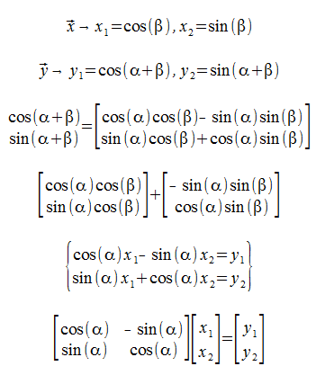
What is the rotation matrix?

Matrix of a Linear TF

Theorem

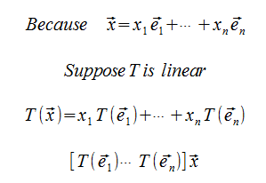
Let T: Rⁿ → R^m be a linear transformation, then there exists a unique matrix A such that T(x) = Ax

Moreover, if e_j denotes the j^th-column of the nxn identity matrix I, then A = [T(e₁) ... T(e_n)].

We're stating that any Linear transformation is (and thus can be written as) a Matrix Transformation.

Proof

Matrix Operations

• Main Diagonal
• Off Diagonal Entries
• Diagonal Matrix
• Zero Matrix

Matrix Algebra

Algebraic operations on matricies are defined by keeping in mind that T(x) = Ax.

Equality

For matricies A and B, say that A = B if a_ij == b_ij.

Consequnce: A = B → A and B have the same size.

Addition

For mxn matricies A and B, the sum f A and B (A+B) is the mxn matrix whose (i,j)-entry is a_ij + b_ij.

Matricies of inequal dimensions is not defined.

Scaling

For A an mxn matrix, the matrix rA (where r is in R), is the mxn whose (i,j)-entry is r * a_ij.

Negative Unary

Defined as -A = -1 * A

Subtraction

Defined as A-B = A + (-B)

Hadamard Product

Multiplying matrices A and by doing: a_ij * b_ij.

Multiplication

If A is an mxn matrix, B is an nxp matrix, then AB = [Ab₁ ... Ab^p]

Transpose

For A, an mxn matrix, define the "Transpose of A", denoted by A^T, is the nxm matrix whose (i, j) entry is a_ji.

This just turns the rows in A into columns.

(A^T)^T = A

(A+B)^T = A^T + B^T

(rA)^T = r(A^T)

(AB)^T = B^T A^T

Theorem

If A, B, and C are matricies, and r, s are scalars, then...

• A+B = B+A (Commutative)
• (A+B)+C = A+(B+C) (Associative)
• A+0 = 0+A = A
• r(A+B) = rA + rB
• (r+s)A = rA + sA
• r(sA) = (rs)A

Why is matrix multiplication the way it is?

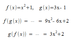
Based on the idea of function composition. For example, f(x) = y, and g(y) = z, thus g(f(X)) = z!

Now let's examine two Matrix transformations that map a vector x from Rⁿ to R^m with some matrix A, and then that result can get mapped to R^p with some matrix B! This looks a lot like function composition.

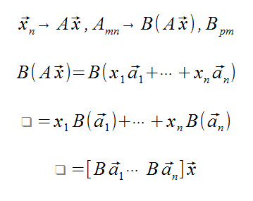
Notice the first transformation is the last matrix (B in this case), just like function composition!

Not only is BA ≠ AB, but in some cases, BA may be undefined!

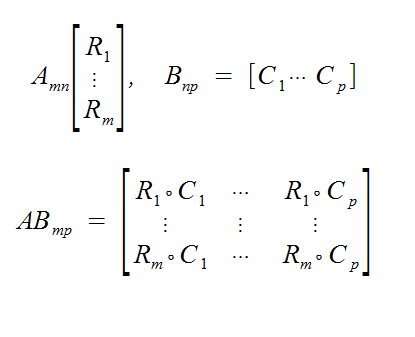
Row-Column Rule

Define vector dot products as the sum of multiplying two vectors entry-wise. x dot y = sum (from 1 to n) of (x_i * y_i)

Theorem

• We can do associative things with matrix multiplication. A(BC) = (AB)C
• A(B+C) = AB + AC. (Left Distributive)
• (B+C)A = BA + CA. (Right Distrbutive)
• r(AB) = (rA)B = a(rB)
• Identitiy Matrix I, I_mA = A = AI_n

Notice that A(B+C) = AB + AC, and (B+C)A = BA + CA, but we cannot say that A(B+C) = BA + CA!

Powers of matricies

Suppose that A is a square matrix, then the following are defined: AA, A(AA), (AA)A. They are commutative too!

Therefore, we define A² as AA, and a³ as A(AA), and so on.

A^k = A*A*A ...

And now then, A^k * A^l = A^{k + l} if k and l are greater than 1.

For convienience, we define A¹ as A. And A⁰ as the identity matrix.

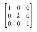
Multiplying by diagonal matricies

If A is some matrix, and D is some disagonal matrix, then:

• AD results in A's columns getting scaled by the appropriate entry in D.
• DA results in A's rows getting scaled by the appropriate entry in D.

Matrix Inverse

Does there exist a matrix B such that B(Ax) = x for any x?

• Inverse Matrix

The Matrix B is unique.

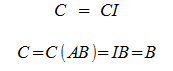
Assume there's a matrix C, not equal to B, such that AC = CA = I.

Why must it be square?

One could say that an mxn matrix A is invertible if there exists nxm matricies C and D such that CA = I_n and AD = I_m. However, these equations imply that A is square and C = D.

Find a 2x2 Inverse Matrix

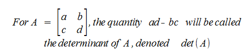
Theorem

If A is a 2x2 matrix, then ad-bc (product of diagonal entries minus product of non-diagonal entries) ≠ 0, then A is invertible and:

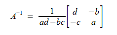
Conversely, if the scenario above is equal to 0, then A is not invertable.

A matrix A is invertible if, and only if, the vectors making up the matrix form a linearly independent set!

Example

Determine if A is invertible, and if it is, find the inverse.

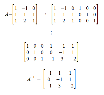
Theorem

If A is an nxn matrix, then A is invertible if, and only if, [A|I] ~ [I|B], therefore A is invertible iff A ~ I, and its inverse is B.

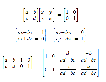
Setup

If A is an nxn matrix, then A is invertible iff there exists an nxn matrix X = [x₁, ..., x_n] such that AX = I.

• ↔ A[x₁, ..., x_n] = [e₁, ..., e_n]
• ↔ [Ax₁, ..., Ax_n] = [e₁, ..., e_n]
• ↔ Ax₁ = e₁, ..., Ax_n = e_n are feasible

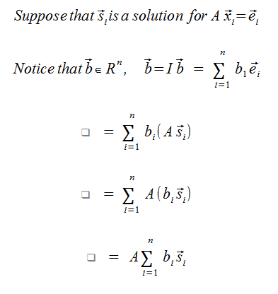
Lemma

(a "Lemma" doesn't look like much, but still acts like a theorem and can have big implications.)

If Ax_i = e_i is consistent for every i from 1 to n, then the linear system Ax = b is feasible for every vector b in Rⁿ.

Proof

Following the set-up and the Lemma, A is invertible iff Ax = b is feasible for every b in Rⁿ, which is to say, A is invertible iff A has a pivot in every row.

Theorem

• If A is invertible, then (A^-1)^-1 = A
• Because -1 * -1 = 1, and A¹ = A
• If A and B are invertible, then AB is invertible and (AB)^-1 = B^-1A^-1
• Because in matrix transformations, we do B and then A, so to undo this we have to undo B first, then undo A.
• If A is invertible, A^T is invertible, and (A^T)^-1 = (A^-1)^T.
• If k is any natrual number, then A^-k = (A^k)^-1.

Invertible Matrix Theorem

Let A be an nxn matrix, Then the following are equivalent (all true or all false)

• A is invertible.
• A is row-equivalent to the Identitiy.
• Any ecehlon form of A has n pivot positions.
• Ax = 0 has only the trivial solution.
• The columns of A are linearly independent.
• Ax = b is consistent for every vector b in Rⁿ
• The span of the columns of A cover all of Rⁿ
• There exists a matrix C such that CA = I.
• There exists a matrix D such that AD = I.
• A^T is invertible.
• The determinant of A is not 0.
• 0 is not an eiganvalue of A.

Theorem

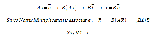
If A and B are square matricies, such that AB = I, then BA = I.

Proof

(Claims)

1. The columns of AB are Linearly Independent.
2. The columns of B are Linearly Independent.
3. The columns of A are L.I.
4. BA - I = 0.

Claim 1: If not, there exists a non-zero vector x such that (AB)x = 0, but (AB)x = Ix = x, thus a contradiction.

Claim 2: If not, there exists a non-zero vector x such that (B)x = 0, but (AB)x = A(Bx) = A(0) = 0 = x (from previous claim).

Claim 3: If not, there exists a non-zero vector y such that Ay = 0. Since Bx is feasible for every vector b in Rⁿ, then there is a non-zero vector x such that Bx = y. Now, 0 = Ay = A(Bx) = (AB)x = x, thus a contradiction.

Claim 4: AB = I, so ABA = A, so A(BA-I) = 0. If not, then BA-I has a nonzero entry and hence a non-zero column. This can't happen because A is L.I.

Elementary Matricies

• Elementary Matricies

Wouldn't it be nice to find a matrix to simplify our row-operations?

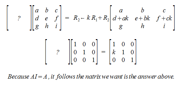
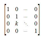
Adding rows by some scalar:

Row Interchange:

Row Scaling:

Matrix Factorizations

• Triangluar Matrix
• Factor

Theorem

If A is an nxn triangular matrix (upper, lower, or both), then A is invertible ↔ every diagonal entry is non-zero. (Obvious Proof)

Proposition

If A and B are square lower triangular matricies, then AB is lower triangular. Same for upper triangular.

Why Factor?

What's is the most efficient way to solve A x₁ = b₁, A x₂ = b₂, etc...

Direct correlation to processing verticies and graphics!

Fact

If Elementary matrix that corresponds to Row Replacement (Adding with a scalar multiple of another row), then E^-1 exists with -k nistead of k.

LU-Factorization

Theorem

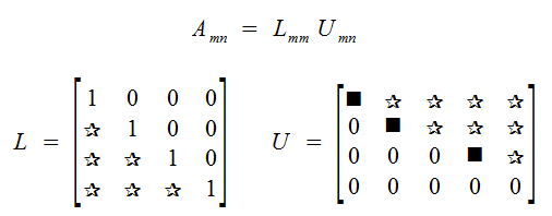
If A is an mxn matrix that can be row-reduced to echelon form without row interchanges, then there is an mxm unity lower triangular matrix L, and an echelon matrix U of A such that A = LU.

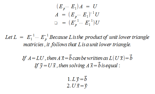
Proof

By Hypothesis, there exists lower-triangular matricies E₁, ..., E_p (corresponding to Row Replacements) such that (E_p ... E₁) A = U.

How do it?

• Only use Row Replacements (Row + c * otherRow)
• Only use Rows below the row you're replacing (creating upper triangle)

1. Reduce A to an echelon form U using the rules above
2. Place the entries in L such that the same sequence of row operations reduces L to I.

Subspaces of Rⁿ

• Vector Space
• Subspace

Any plane in R³ that contains the zero-vector, will look and act like R².

Theorem

Proof

• Clearly the zero vector is in the span.
• Suppose that u and v are in the span of V, thus there is a Linear Combo of V to result in u and v.
• Clearly u+v are in the span as well.
• And again, we can scale the vector u and this is also in the span.

IS there a span in Rⁿ that is not a subspace?

Fundamental Subspaces of a Matrix

• Columnspace
• Nullspace

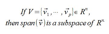
If A is an mxn matrix, then Col(A) is a subspace of R^m (because, as we stated above in the theorem, a span of vectors is a subspace).

If A is an mxn matrix, then the Nulspace of A is a subspace of Rⁿ (not m!).

Basis

A basis for a subspace H of Rⁿ is a linearly independent set in H that spans H.

The columns of the nxn identity matrix form what's known as the standard basis for R_n.

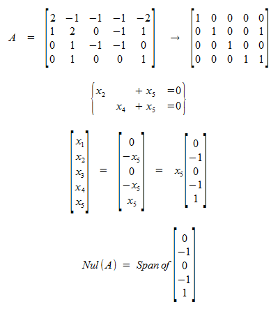
To find a basis for the null space

1. Row-Reduce the matrix A with the homogenous form (Ax = 0) to its Reduced Echelon Form
2. Put the solution set in parametric vector equation form to get your Linearly Independent Spanning Set.

Example:

To find a column basis

1. Bring a matrix to its Reduced Echelon Form.
2. Each pivot column in the matrix means the corresponding column (vector) in the original matrix will form the basis for the Column Space.

Why is not the R.E.F. matrix's columns that are the basis, but the original matrix's?

Row operations change the column space, but the solutions (in terms of generic vectors of the Linear System) remain the same.

Dimension of a Matrix

First off, let's define the word "dimension&qout;.

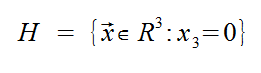
We'd like to say that the dimension of H is 2, even though it lives in R³.

Theorem

Let H be a subspace of Rⁿ and let B (a set of vectors) be a basis for H.

If vector x is in H, then there are unique scalars such that the vector x can be written as a linear combination of the vectors of B.

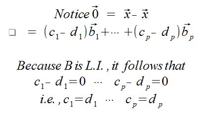
Proof

Because B is a spanning-set, the existance of these scalars is guaranteed. Now, for uniqueness... Assume there are another set of scalars where at least one is not equal to the previously stated scalars, such that these scalars can be written as a linear combination of the vectors of B.

For every vector x in H, the coordinates of x relative to B are the unique scalars such that x = Bc.

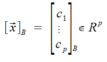
The vector x (as above) is called the B-coordinate vector of the original vector x.

So what is this mess?

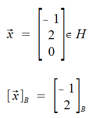
Imagine H as the the image above in this section. A basis for H is the 3x3 Identitiy matrix with the 3rd column 0.

We can use the definition above to say:

Consider the correspondence f: H → R^p where vector x → [x]_B.

It can be shown that f is a bijective mapping that preserves linear combinations. This means the function is linear (so you can use algebra happily).

Such a mapping is called an isomorphism, and we say that H and R^p are isomorphic (Same Structure). This is the mathematical precision of saying "H looks and acts like R², so we can just go play in R² and be happy.

Remark

Because there infinitely many bases for H, and the dimension we isomorph H into depends on the number of vectors in the base, how can we truly say H is an isomorph of R^p. Well, a basis has to be a Linearly Independent set, so therefore it will always have the same number of vectors.

Convention

The dimension of the zero-vector is equal to 0.

Rank of a Matrix

• Rank
• Nullity

Consider a 3x5 matrix with pivot columns in 1 and 3. The Rank(A) = 2. Nullity(A) = 3.

Theorem

If A is an mxn matrix, then the rank(A) + nullity(A) = m

Determinants

Recall the solution for determining if a 2x2 matrix is invertible.

• Invertible can be called non-singular
• Non-Invertible can be called singular

Now, wouldn't it be nice if there is a determinant for matrices that are not 2x2? Calculating them is way too complex though. Forexample, the determinant for a 3x3 is:

2x2 had 2 terms, 3x3 has 6 terms... Calculating the determinant requires n-factorial terms, which is the worst big-O ever!

Anyway, notice that A is invertible iff det(A) ≠ 0.

The ugly terms above can be rewritten like so:

Notice that within each parenthesis, the determinant depends on the determinants of the 3 unique 2x2 sub-matrices!!

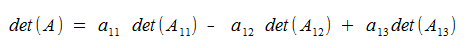
Where A_ij is the matrix obtaind from A by deleting the i^th row and the j^th column of A.

size(A_ij) is (n-1) x (n-1)

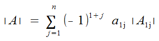
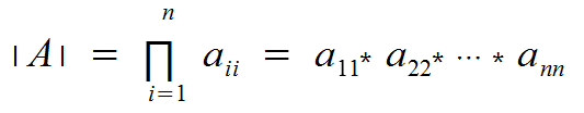
For n >= 2, the determinant of the nxn matrix of A [a_ij], denoted by det(A), or delta_A, or |A|, is given by:

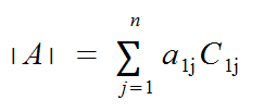
Using Cofactors, we can rewrite this more simply.

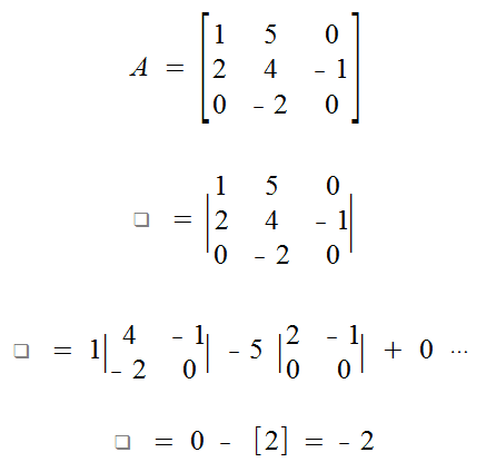
Example

Find det(A).

Theorem

If A = [a_ij] is an nxn matrix, then we can take a determinant with either the rows or the columns.

• A determinant by going across a row is called: a cofactor expansion across row i.
• A determinant by going down a column is called: a cofactor expansion down column j.

You can actually use any row and column to "go along"!

The 1's listed above in the equation for a determanent can be repalced with i to indicate a row. The i-variable never changes through the summation though, so it's fixed.

Notice that Triangular Matricies make this easier

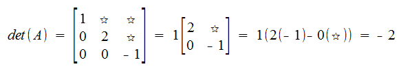
Theorem

If A is triangular (upper or lower) then:

The problem is that row operations change the column space of the matrix, so even though we can make a triangular matrix, we can't use that to calculate the determinant.

Properties of Determinants

How do Row-Ops Affect Determinant?

2x2 Matricies

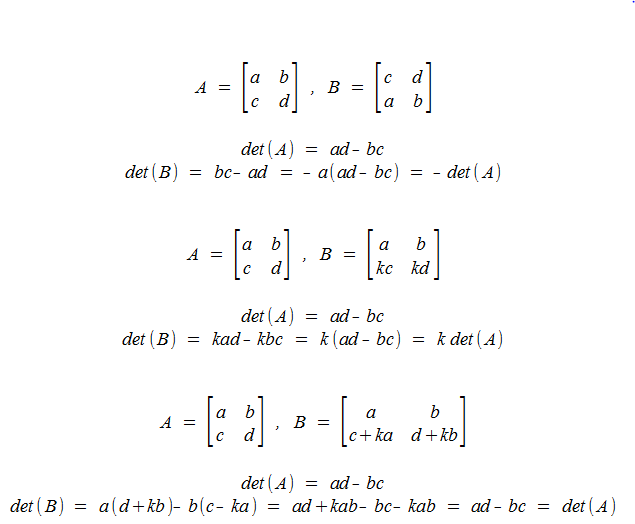
• If A~B via R_i ↔ R_j, then - det(A) = det(B)
• If A~B via R_i ← kR_i, then k det(A) = det(B)
• If A~B via R_i ↔ R_i + k R_j, then det(A) = det(B)

Example

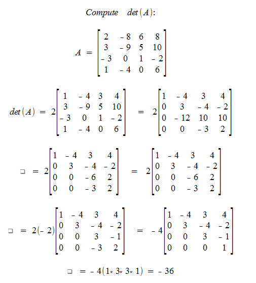
A faster way to calculate the determinant

Suppose that a square matrix A has been row-reduced to an echelon form U via row-replacements (R becomes R + k someOtherRow) and row-interchanges (which is always possible). If there are r row-interchanges performed, then det(A) = (-1)r det(U)!

Because U is upper-triangluar, if follows that the determinant of U is the product of its diagonal entries.

If U is invertile, then its diagonal entries are all non-zero, and if U is non-invertible, then there must be at least one zero value in the diagonal entries.

Theorem

The square matrix A is inverible iff det(A) ≠ 0

Theorem

If A is an nxn matrix, then det(A) = det(A^T). Intuitively, this is because if you calculate the determinant by going down A's j^th column, this is equal to calculating the determinant by going down A^T's j^th row.

Theorem

If A and B are square matricies of the same size, then det(AB) = det(A) det(B).

Maths

• det(AB) = det(A) * det(B)
• det(A+B) ≠ det(A) + det(B)

Eigenvectors & Eigenvalues

Why are these important?

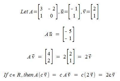
Notice that the mapping Av is just scalaing the vector v by 2! This is just weird, given this doesn't happen for other vectors (like u).

This also means any scalar of v will get scaled by 2 when mapped by A, so the Eigenspace is the vector v.

• Eigenvector
• Eigenvalue

The definition of Eigenvector and Eigenvalue means that for one eigenvalue, there may be multiple eigenvectors. As in the example above, any scalar of v is an acceptable eigenvector for the eigenvalue 2.

Now, are there multiple eigenvalues for a single eigenvector? No, because by the definition, Ax = lx, so having Ax also = ux, is impossible.

Example

Verify that 7 is an eigenvalue for:

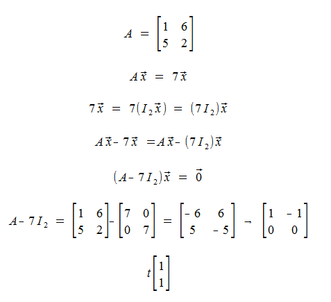
Any vector of the form t, is an eigenvector corresponding to 7.

Theorem

From the previous example, notice that lambda is an eigenvalue for A iff the Homogeneous Linear System (A - lambda I_n)x = 0 has a nontrivial solution.

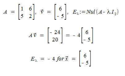
The set of all solutions to this H.L.S., is the Nullspace of that equation: Nul(A - lambda I_n) and this is called the eigenspace of A corresponding to lambda.

Example

Example

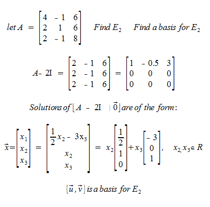
Theorem

The eiganvalues of a triangular matrix are its diagonal entries.

Proof

Consider the upper-triangular case. If A is an upper triangluar matrix, then A - lambda I, results in a_nn - lambda for all diagonal entries. The upper entries in A don't change, and the 0s below remain 0.

Thus, (A - lambda I) has a nontrivial solution iff a_ii - lambda ≠ 0. And further, a_ii is an eiganvalue for A. This also works for lower triangular matricies.

We cannot use row operations to make a matrix into a triangle form to get its eiganvalues, because row operations ruin the original matrix's eiganvalues.

Theorem

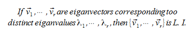
Proof

Assume that there exists scalars, such that a linear combination of some of the vectors of v with respect to the scalars, results in a vector already in the set. This means one of the vectors in v is a linear combination of the others, so it's extra, so v would be L. D.

From here, basically we play with it by multiplying it by the matrix A and substituing lambda, and it results in a contradiction where it states that one of the vectors in v must be 0, which we already said wasn't true.

The Characteristic Equation

Given an nxn matrix A, how do we compute its eiganvalues? Use the determinant of A to test for invertiblity, and thus for non-trivial solutions of Nul(A - lambda I)!

It is sometimes better to express it as: Nul(lambda I - A).

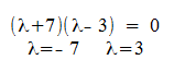
Example

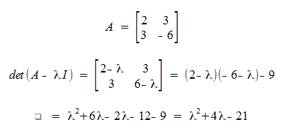
Thus Lambda is an eiganvalue of A iff:

• Finding the eiganvalues of a 2x2 matrix is equivalent to solving a quadratic equation.
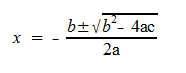
• The soltions of ax²+bx+c = 0 (where A > 0 (actually a is always 1 for us!)) are given explicitly by the quadratic formula

Example

• Characteristic Equation

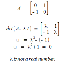
nxn matricies have exactly n eigan values. This is proved by showing that the characteristic equation boils down to a polynomial of the n^th degree, and there is a proof that a polynomial of n-degrees has exactly n roots. This means the characteristic equation has n roots.

However, Galois Theory states that degrees of 5 or higher cannot be expressed like a quadratic equation, so actually the eiganvalues of an nxn matrix cannot be computed explicitly.

Characteristic Polynomial

Rather than state the determinant of lambda I - A to 0 to solve for a particular eiganvalue, we call lambda 't', and don't set it to 0 explcitly. This results in a polynomial with varius t variables and makes it really easy to see which values will result in the equation being 0.

Matrix Similarity

A special group of matricies:

further, if A and B are similar, then A and B have the same eigenvalues!

This is the technique used to find eigenvalues of large matricies because we can't express large matricies as a polynomial (easily).

Diagonalization

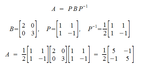
A fundamental goal in matrix theory is to write most matricies in the form P D P^-1, where D is a diagonal matrix. Most matricies are similar to a diagonal matrix.

• Diagonalization

This is super cool, because if we're doing a mapping with a vector x, then we're mapping x to a different basis (P^-1), then hit it with a diagonal matrix (super easy to calculate and see what it does), then map it back to its original space wth P!

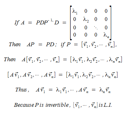
Theorem

A is diagonalizable iff A has n linearly independent eiganvectors. Morever, A = PDP^-1, iff the columns of P are n linearly independent eigenvecotrs of A. The diagonal entries of D are the eiganvalues of A.

Proof

This argument can be proven by reversing the argument above, so it's an iff.

Example

Diagonalize (if possible) the matrix:

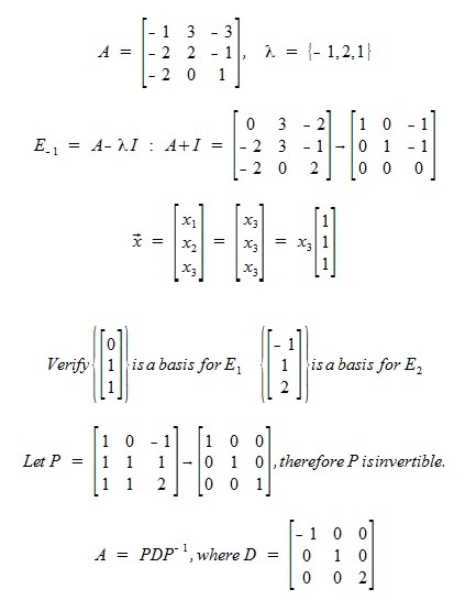
Note that we can create P by setting the eiganvectors in any order. Just as long as the order of the eiganvectors match the order of the eiganvalues.

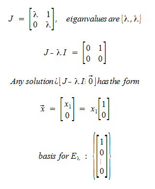
Example

Non-diagonalizable matrix (Jordon Block).

Theorem

An nxn matrix with n distinct eiganvalues is diagonalizable. HOWEVER, if an nxn matrix is diagonalizable, it does not contain distinct eiganvalues.

Proof

Follows the prooof way above that states if there is a lineraly indepent set of eigan vectors, then there is a L.I. set of eiganvalues, thus can be diagonalized.

Length

Length in R² is easy, d² = sqrt(a² + b²), but for any dimensional space, how do we get the length of a vector?

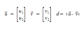
Distance in Rⁿ

Inner Product

Also called the dot product, is the product of a vector u and v, calcuated by u^Tv. The result is a scalar (R¹).

For the purposes of this kind of multiplcation, we call vectors an nx1 matrix, so that u^Tv is a matrix multiplcation, which results in a 1x1 matrix, or a scalar.

Theorem

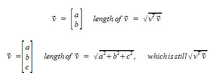
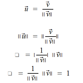
For a vector v, a column vector, we define the length (norm) of v as the nonnegative quantity ||V|| = sqrt(v^T v)

Proposition

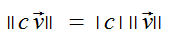
If vec v is a column vector, and c is any real number, then

• Norm
• UnitVector

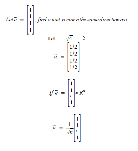
If vec v is any nonzero vector, thenthe length of a vector u is one by this:

Matricies and Vectors

Matrices behave like vectors. You can scale them, there's a 0-matrix like the 0-vector, and you can actually define the distace of a matrix...

Orthogonality

We want to generalize the notion of perpendicularity to Rⁿ.

We define two vectors to be othrogonal (based on geometry), as the distance from v to -u must be eqal to the distance from v to u. This is only true if u dot v is 0.

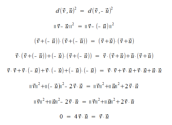
Definition

We say that the vectors u and v of Rⁿ are orthogonal (to each other) if u dot v = v dot u = 0

As a consequence, every vector is orthogonal to the zero-vector.

Now, if u dot v is 0, then any scalar multiple of either u or v must be orthogonal.

Orthogonal Complement

(Reminder) A subspace is a subset within a space that looks and acts like a lower dimension. Note that a subspace of R³ is a set of vectors in R³, but it looks and acts like some unspecified lower dimension. It is still a subspace of R³.

If W i a subspace of Rⁿ, then the orthogonal complement of W, denoted W^⊥, = {vec z in Rⁿ : z dot w = 0, for every w in W}.

• If W is a subspace of Rⁿ
• vec x is in W^⊥ iff x is orthogonal to every vector in a spanning set of W
• W^⊥ is a subspace of Rⁿ
• (W^⊥)^⊥ = W

• In R³, the Perp of a plane is a line, and the perp of a line is a plane.

Orthogonal Sets

A set of vectors {u₁, ..., u_n} in Rⁿ is called orthogonal or an orthogonal set if u_i dot u_j = 0 whenever i ≠ j.

The columns of the identity matrix form an orthogonal set.

Example

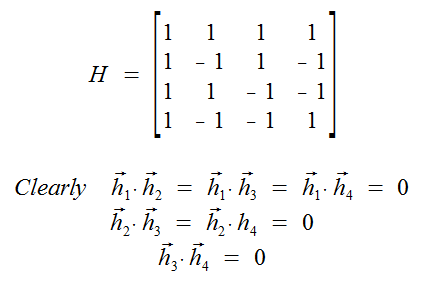
Show that the columns of the Hadamard matrix are orthogonal.

Aside

Hadamard matricies are formed by placing a 1 in a 2x2 matrix, then a -1 in the bottom-right position. To make a bigger matrix, repeat this pattern with this 2x2 matrix to make a 4x4 matrix. Now you could make a 8x8, 16x16...

• H^T H = nI

---

Orthogonal Sets

A set of vectors U is an orthogonal set if u_i dot u_j = 0, whenever i ≠ j.

For example, the columns of the Identity matrix, or the columns of the Hadamard Matrix.

Why does this matter?

If U is orthogonal, then U is Lineraly Independent, and hence a basis for span(U).

Proof

The coverse is clearly not true. Suppose that there are scalars C (not all zero) such that U dot C = 0. (In a L.I. system, only when all scalars are 0 is the solution).

Assume that c_i ≠ 0

Orthogonal Basis

An orthogonal basis is an orothogonal Linearlly Independent Spanning Set.

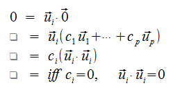
Theorem

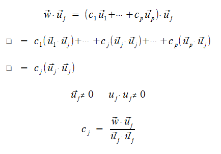
If U is a set of vectors in Rⁿ and is an orthogonal basis, and W is the span(U), then for any vector w in W...

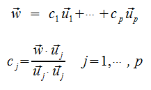
This means we don't have to solve a linear system to find out the scalars for each x.

Proof

Because U is a basis, there are unique scalars C such that vector w = C dot u.

Complexity

This algorithm is linear, wheras solving for non orthogonal matricies, it's exponential! (n³)

Orthonormal Set

An orthogonal set, but the vectors are also all unit vectors. Given an orthogonal set, it's very easy to turn it into an orthonormal set.

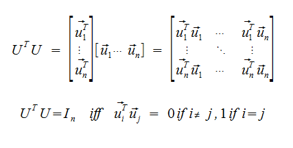
Theorem

If U is an mxn matrix, then U has orthonormal columns iff U^TU = I_n

Proof

---